The PyOPIA Particle STATS#
How to create STATS, how is it structured, and how to plot a volume distribution
Installation note:#
These examples use ‘classification’ optional dependencies, which you should have installed (see here).
The PyOPIA particle classifier#
PyOPIA includes a convolution neural network (CNN) based object/particle classifier. To learn more about it and check its performce, see this notebook.
Process an example image#
First, we can setup and example pre-trained CNN, available from the pyopia.tests module.
model_path = pyopia.exampledata.get_example_model(os.getcwd())
Now we can use a config file to define a set of processing steps for a SilCam image (pyopia.instrument.silcam). You can generate this config file using pyopia generate-config (see the ‘Command line tools’ page for more info), or you could have a look at some of the example config files in the notebooks folder
toml_settings = pyopia.io.load_toml('config.toml')
And run the pyopia.pipeline.Pipeline class
# Initialise the pipeline and run the initial steps
processing_pipeline = pyopia.pipeline.Pipeline(toml_settings)

# Load an image (from the test suite)
filename = pyopia.exampledata.get_example_silc_image(os.getcwd())

# Process the image to obtain the stats dataframe
processing_pipeline.run(filename)
stats = processing_pipeline.data['stats']
Show code cell output
Initialising pipeline
WARNING: Classification assumes loaded images have values in the range 0-255
Classify  ready with: {'model_path': 'keras_model.h5'}  and data dict_keys(['cl', 'settings', 'raw_files'])
Example image already exists. Skipping download.
SilCamLoad  ready with: {}  and data dict_keys(['cl', 'settings', 'raw_files', 'filename'])
ImagePrep  ready with: {'image_level': 'imraw'}  and data dict_keys(['cl', 'settings', 'raw_files', 'filename', 'timestamp', 'imraw'])
Segment  ready with: {'threshold': 0.85}  and data dict_keys(['cl', 'settings', 'raw_files', 'filename', 'timestamp', 'imraw', 'imref', 'imc'])
segment
clean
CalculateStats  ready with: {}  and data dict_keys(['cl', 'settings', 'raw_files', 'filename', 'timestamp', 'imraw', 'imref', 'imc', 'imbw'])
statextract
21.7% saturation
measure
  870 particles found
WARNING. exportparticles temporarily modified for 2-d images without color!
EXTRACTING 870 IMAGES from 870
StatsToDisc  ready with: {'output_datafile': './test'}  and data dict_keys(['cl', 'settings', 'raw_files', 'filename', 'timestamp', 'imraw', 'imref', 'imc', 'imbw', 'stats'])
Note: the returned stats from stats = processing_pipeline.run(filename) are single-image only and not appended if you loop through several filenames! It is recommended to use this step as part of pipeline that uses pyopia.io.StatsToDisc for properly appending data into NetCDF format when processing several files.
The STATS DataFrame#
This is the main Pandas DataFrame containing the processed information about every particle measured.
This does not contain any calibrated values, so dimentions (e.g. equivalent_diameter etc.) and positions of ROI bounding boxes (e.g. minr etc.) are all in pixels (not microns). This allows for altering pixels size without having to re-process if a post-calibration is performed on the data, for example.
The position of each particle within the original raw image are given by the bounding box at location (minr, minc, maxr, maxc) - with r and c being rows and columns, respectively.
Classification probabilities are given by columns with ‘probability_*’. Note: If [steps.classifier]is not defined in the config, the classification will be skipped and no probabilities reported. To use PyOPIA’s Classification module requires the extra dependencies (pip install pyopia[classification] or pip install pyopia[classification-arm64])
# print the stats DataFrame
stats.head()
| major_axis_length | minor_axis_length | equivalent_diameter | minr | minc | maxr | maxc | probability_oil | probability_other | probability_bubble | probability_faecal_pellets | probability_copepod | probability_diatom_chain | probability_oily_gas | export name | timestamp | saturation | |
|---|---|---|---|---|---|---|---|---|---|---|---|---|---|---|---|---|---|
| 0 | 6.175643 | 2.743739 | 3.908820 | 3.0 | 77.0 | 8.0 | 81.0 | 0.285310 | 0.053474 | 5.428675e-01 | 4.880920e-03 | 3.022380e-03 | 4.415022e-03 | 1.060302e-01 | D20181101T142731.838206-PN0 | 2018-11-01 14:27:31.838206 | 21.666268 |
| 1 | 15.518777 | 13.091788 | 14.138550 | 3.0 | 1896.0 | 18.0 | 1912.0 | 0.219160 | 0.005522 | 7.531021e-01 | 2.015659e-06 | 7.330137e-06 | 2.535686e-06 | 2.220398e-02 | D20181101T142731.838206-PN1 | 2018-11-01 14:27:31.838206 | 21.666268 |
| 2 | 21.233102 | 18.983567 | 20.026744 | 4.0 | 181.0 | 26.0 | 202.0 | 0.982581 | 0.000725 | 8.770840e-03 | 5.576220e-08 | 1.831942e-06 | 7.583355e-06 | 7.914181e-03 | D20181101T142731.838206-PN2 | 2018-11-01 14:27:31.838206 | 21.666268 |
| 3 | 37.163209 | 34.977428 | 36.019871 | 4.0 | 282.0 | 41.0 | 318.0 | 0.999999 | 0.000001 | 6.355144e-08 | 5.643562e-11 | 2.458285e-12 | 2.210773e-13 | 6.275302e-10 | D20181101T142731.838206-PN3 | 2018-11-01 14:27:31.838206 | 21.666268 |
| 4 | 7.765540 | 7.365920 | 7.225152 | 4.0 | 1444.0 | 12.0 | 1452.0 | 0.398723 | 0.057881 | 4.832646e-01 | 2.050719e-03 | 4.557050e-03 | 4.770531e-03 | 4.875316e-02 | D20181101T142731.838206-PN4 | 2018-11-01 14:27:31.838206 | 21.666268 |
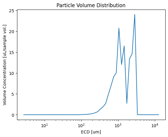
Analysis, statistics and plotting#
There are lots of functions in pyopia.statistics. Here is just an example using pyopia.statistics.vd_from_stats()
# Calculate the volume distribution from the stats DataFrame.
# (Usually several images would be needed for statistics to converge.
# This can be done by appending new image stats to the DataFrame)
dias, vd = pyopia.statistics.vd_from_stats(stats, 24)

# plot the volume distribution
plt.plot(dias, vd)
plt.xscale('log')
plt.xlabel('ECD [um]')
plt.ylabel('Volume Concentration [uL/sample vol.]')
plt.title('Particle Volume Distribution')
plt.show()