Running steps manually & add-hoc operations#
Installation note:#
These examples use ‘classification’ optional dependencies, which you should have installed (see here).
Initial admin#
# get an image and filename for working on in this example
filename = pyopia.exampledata.get_example_silc_image(os.getcwd())

# Initial start of the settings, which will be added to as we go
settings = {'general': {'raw_files': None,
                        'pixel_size': 24},
            'steps': {'note': 'non-standard pipeline.'}
           }

# Initialise the pipeline class without running anything
MyPipeline = pyopia.pipeline.Pipeline(settings=settings, initial_steps='')
Example image already exists. Skipping download.
Initialising pipeline
Setup classification#
This is the first pipeline step top run. We will first define in the settings dictionary (as we would normally do in the toml file). Then we execute the step using Pipeline.run_step().
We could call the method directly and skip the settings definitions, but by first defining the setup within the settings[‘steps’], we ensure that the metadata description of the pipeline matches what we have actually done.
# Get the example trained model
model_path = pyopia.exampledata.get_example_model(os.getcwd())

# Add the classifier step description to settings (i.e. metadata)
MyPipeline.settings['steps'].update({'classifier':
                                       {'pipeline_class': 'pyopia.classify.Classify',
                                       'model_path': model_path}
                                    })

# Execute the classifier step we defined above
MyPipeline.run_step('classifier')
# This is the same as running:
# MyPipeline.data['cl'] = pyopia.classify.Classify(model_path=model_path)
# Note: the classifier step is special in that it's output is specifically data['cl'], rather than other new keys in data

MyPipeline.data
WARNING: Classification assumes loaded images have values in the range 0-255
Classify  ready with: {'model_path': 'keras_model.h5'}  and data dict_keys(['cl', 'settings', 'raw_files'])
{'cl': <pyopia.classify.Classify at 0x1057183d0>,
 'settings': {'general': {'raw_files': None, 'pixel_size': 24},
  'steps': {'note': 'non-standard pipeline.',
   'classifier': {'pipeline_class': 'pyopia.classify.Classify',
    'model_path': 'keras_model.h5'}}},
 'raw_files': None}
Load an image#
# Since we are not going to be using MyPipeline.run(filename) here, we need to manually add filename into the pipeline data:
MyPipeline.data['filename'] = filename

# Add the load step description
MyPipeline.settings['steps'].update({'load':
                                       {'pipeline_class': 'pyopia.instrument.silcam.SilCamLoad'}
                                    })

# Run the step
MyPipeline.run_step('load')
# This is the same as running:
# SilCamLoad = pyopia.instrument.silcam.SilCamLoad()
# MyPipeline.data = SilCamLoad(MyPipeline.data)

plt.imshow(MyPipeline.data['imraw'][:,:,:]/255)
plt.title('imraw')
SilCamLoad ready with: {} and data dict_keys(['cl', 'settings', 'raw_files', 'filename'])
Text(0.5, 1.0, 'imraw')
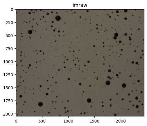
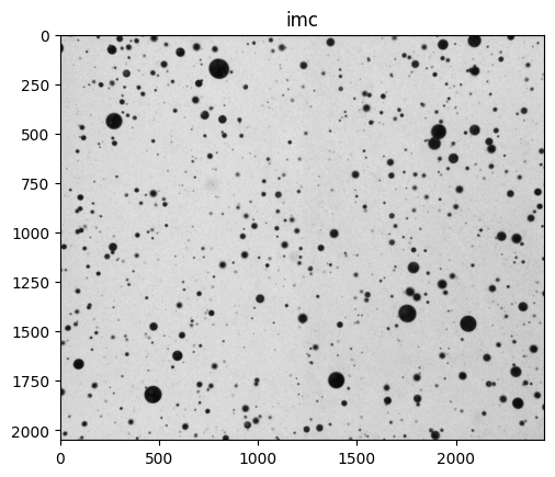
Image preparation#
# Add the imageprep step description
MyPipeline.settings['steps'].update({'imageprep':
                                       {'pipeline_class': 'pyopia.instrument.silcam.ImagePrep',
                                        'image_level': 'imraw'}
                                    })
# Run the step
MyPipeline.run_step('imageprep')
# This is the same as running:
# ImagePrep = pyopia.instrument.silcam.ImagePrep(image_level='imraw')
# MyPipeline.data = ImagePrep(MyPipeline.data)

plt.imshow(MyPipeline.data['imc'], cmap='grey')
plt.title('imc')
ImagePrep ready with: {'image_level': 'imraw'} and data dict_keys(['cl', 'settings', 'raw_files', 'filename', 'timestamp', 'imraw'])
Text(0.5, 1.0, 'imc')
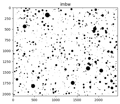
Segmentation#
# Add the segmentation step description
MyPipeline.settings['steps'].update({'segmentation':
                            {'pipeline_class': 'pyopia.process.Segment',
                            'threshold': 0.85}}
                        )
# Run the step
MyPipeline.run_step('segmentation')
# This is the same as running:
# Segment = pyopia.process.Segment(threshold=settings['steps']['segmentation']['threshold'])
# data = Segment(data)

plt.imshow(~MyPipeline.data['imbw'], cmap='grey')
plt.title('imbw')
Segment  ready with: {'threshold': 0.85}  and data dict_keys(['cl', 'settings', 'raw_files', 'filename', 'timestamp', 'imraw', 'imref', 'imc'])
segment
clean
Text(0.5, 1.0, 'imbw')
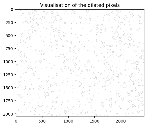
Insert an add-hoc step#
Let’s write some custom code that is used as an add-hoc step in the middle of a pipeline.
Here we will add a 1-pixel dilation around all particles using skimage. We will still describe the step in the settings (metadata), so it is recorded together with the data
# Define a step for inserting into the metadata.
MyPipeline.settings['steps'].update(
                    {'dilation':
                        {'custom step': 'dilate segmented image by 1 pixel'}}
                )

# run our custom code
import skimage

imbw_original = MyPipeline.data['imbw']
imbw_dilated = skimage.morphology.binary_dilation(imbw_original)

plt.imshow(imbw_original.astype(int) - imbw_dilated.astype(int), cmap='grey')
plt.title('Visualisation of the dilated pixels')

# redefine 'imbw', which is needed for the next step
MyPipeline.data['imbw'] = imbw_dilated
# Add the segmentation step description
MyPipeline.settings['steps'].update({'statextract':
                                        {'pipeline_class': 'pyopia.process.CalculateStats'}}
                                    )

# Run the step
MyPipeline.run_step('statextract')
# This is the same as running:
# CalculateStats = pyopia.process.CalculateStats()
# data = CalculateStats(data)
CalculateStats  ready with: {}  and data dict_keys(['cl', 'settings', 'raw_files', 'filename', 'timestamp', 'imraw', 'imref', 'imc', 'imbw'])
statextract
24.8% saturation
measure
  853 particles found
WARNING. exportparticles temporarily modified for 2-d images without color!
EXTRACTING 853 IMAGES from 853
Output data#
Make an xarray of the processed data and metadata, which is conforming to the output PyOPIA gives from running a pipeline
xstats = pyopia.io.make_xstats(MyPipeline.data['stats'], settings)
xstats
<xarray.Dataset>
Dimensions:                     (index: 853)
Coordinates:
  * index                       (index) int64 0 1 2 3 4 ... 848 849 850 851 852
    time                        (index) datetime64[ns] 2018-11-01T14:27:31.83...
Data variables: (12/17)
    major_axis_length           (index) float64 7.811 17.56 23.1 ... 8.056 7.524
    minor_axis_length           (index) float64 4.533 14.91 ... 6.461 4.763
    equivalent_diameter         (index) float64 5.863 16.12 ... 7.225 5.971
    minr                        (index) float64 2.0 2.0 ... 2.032e+03 2.036e+03
    minc                        (index) float64 76.0 1.895e+03 ... 1.753e+03
    maxr                        (index) float64 9.0 19.0 ... 2.04e+03 2.044e+03
    ...                          ...
    probability_copepod         (index) float64 0.004393 2.323e-06 ... 0.002888
    probability_diatom_chain    (index) float64 0.003636 2.031e-07 ... 0.003968
    probability_oily_gas        (index) float64 0.06183 0.008561 ... 0.03824
    export name                 (index) object 'D20181101T142731.838206-PN0' ...
    timestamp                   (index) datetime64[ns] 2018-11-01T14:27:31.83...
    saturation                  (index) float64 24.77 24.77 ... 24.77 24.77
Attributes:
    steps:           [general]\npixel_size = 24\n\n[steps]\nnote = "non-stand...
    Modified:        2024-08-09 13:10:53.817878
PyOpia version: 1.1.4- index: 853
- index(index)int640 1 2 3 4 5 ... 848 849 850 851 852
array([ 0, 1, 2, ..., 850, 851, 852])
- time(index)datetime64[ns]2018-11-01T14:27:31.838206 ... 2...
array(['2018-11-01T14:27:31.838206000', '2018-11-01T14:27:31.838206000',
       '2018-11-01T14:27:31.838206000', '2018-11-01T14:27:31.838206000',
       '2018-11-01T14:27:31.838206000', '2018-11-01T14:27:31.838206000',
       '2018-11-01T14:27:31.838206000', '2018-11-01T14:27:31.838206000',
       '2018-11-01T14:27:31.838206000', '2018-11-01T14:27:31.838206000',
       '2018-11-01T14:27:31.838206000', '2018-11-01T14:27:31.838206000',
       '2018-11-01T14:27:31.838206000', '2018-11-01T14:27:31.838206000',
       '2018-11-01T14:27:31.838206000', '2018-11-01T14:27:31.838206000',
       '2018-11-01T14:27:31.838206000', '2018-11-01T14:27:31.838206000',
       '2018-11-01T14:27:31.838206000', '2018-11-01T14:27:31.838206000',
       '2018-11-01T14:27:31.838206000', '2018-11-01T14:27:31.838206000',
       '2018-11-01T14:27:31.838206000', '2018-11-01T14:27:31.838206000',
       '2018-11-01T14:27:31.838206000', '2018-11-01T14:27:31.838206000',
       '2018-11-01T14:27:31.838206000', '2018-11-01T14:27:31.838206000',
       '2018-11-01T14:27:31.838206000', '2018-11-01T14:27:31.838206000',
       '2018-11-01T14:27:31.838206000', '2018-11-01T14:27:31.838206000',
       '2018-11-01T14:27:31.838206000', '2018-11-01T14:27:31.838206000',
       '2018-11-01T14:27:31.838206000', '2018-11-01T14:27:31.838206000',
       '2018-11-01T14:27:31.838206000', '2018-11-01T14:27:31.838206000',
       '2018-11-01T14:27:31.838206000', '2018-11-01T14:27:31.838206000',
...
       '2018-11-01T14:27:31.838206000', '2018-11-01T14:27:31.838206000',
       '2018-11-01T14:27:31.838206000', '2018-11-01T14:27:31.838206000',
       '2018-11-01T14:27:31.838206000', '2018-11-01T14:27:31.838206000',
       '2018-11-01T14:27:31.838206000', '2018-11-01T14:27:31.838206000',
       '2018-11-01T14:27:31.838206000', '2018-11-01T14:27:31.838206000',
       '2018-11-01T14:27:31.838206000', '2018-11-01T14:27:31.838206000',
       '2018-11-01T14:27:31.838206000', '2018-11-01T14:27:31.838206000',
       '2018-11-01T14:27:31.838206000', '2018-11-01T14:27:31.838206000',
       '2018-11-01T14:27:31.838206000', '2018-11-01T14:27:31.838206000',
       '2018-11-01T14:27:31.838206000', '2018-11-01T14:27:31.838206000',
       '2018-11-01T14:27:31.838206000', '2018-11-01T14:27:31.838206000',
       '2018-11-01T14:27:31.838206000', '2018-11-01T14:27:31.838206000',
       '2018-11-01T14:27:31.838206000', '2018-11-01T14:27:31.838206000',
       '2018-11-01T14:27:31.838206000', '2018-11-01T14:27:31.838206000',
       '2018-11-01T14:27:31.838206000', '2018-11-01T14:27:31.838206000',
       '2018-11-01T14:27:31.838206000', '2018-11-01T14:27:31.838206000',
       '2018-11-01T14:27:31.838206000', '2018-11-01T14:27:31.838206000',
       '2018-11-01T14:27:31.838206000', '2018-11-01T14:27:31.838206000',
       '2018-11-01T14:27:31.838206000', '2018-11-01T14:27:31.838206000',
       '2018-11-01T14:27:31.838206000'], dtype='datetime64[ns]')
- major_axis_length(index)float647.811 17.56 23.1 ... 8.056 7.524
array([ 7.81099616, 17.56209232, 23.09893705, 38.98302787, 9.84092426, 7.10288843, 9.31521345, 28.80881657, 9.87486952, 48.50059258, 32.39163839, 7.9917378 , 16.30109045, 58.39167261, 16.06879006, 22.6117302 , 8.15696525, 8.38787781, 19.11884429, 26.92604764, 46.22449601, 15.59680936, 15.42714049, 35.89949967, 43.80107663, 35.20413018, 55.63199911, 17.04035777, 37.58156981, 12.32686057, 23.19831525, 51.58477061, 8.87789446, 24.63689449, 18.50830863, 18.24955987, 8.84446797, 9.18006548, 11.15270745, 9.19330825, 65.09274008, 12.72643498, 18.93619997, 9.84815733, 28.25234516, 19.86148304, 6.91628627, 32.71262808, 7.38419365, 16.53559979, 27.42939529, 11.01941657, 27.37908944, 13.22622213, 11.67816018, 117.94409326, 14.37667321, 10.34405727, 45.13089038, 10.12539565, 40.49105824, 43.58585721, 31.25855705, 13.00220105, 9.78613966, 15.04181892, 11.03134043, 11.66045896, 69.31460016, 8.76564623, 8.28486945, 8.60295358, 15.37580316, 9.33840867, 28.17561715, 11.41839046, 15.96125842, 10.41949763, 17.99170873, 44.0117065 , ... 7.79358494, 20.50233957, 5.99387125, 8.15761958, 9.10551898, 13.13661968, 43.10789658, 13.46554188, 6.73485123, 20.82069085, 8.1722232 , 17.51588946, 15.50736935, 29.29861096, 10.03213039, 13.52097789, 22.69853374, 9.83282871, 8.15104714, 29.49692426, 11.60983464, 11.16020005, 7.37266443, 62.31442003, 19.13818412, 15.19841599, 20.80217388, 21.45012931, 23.08961355, 16.65424679, 17.24332766, 19.54585963, 34.78973456, 16.74411801, 47.04741873, 16.93292998, 22.56383766, 35.06665999, 46.90098828, 11.8650105 , 40.97810523, 20.40889368, 14.88461964, 41.33957636, 15.1230597 , 37.66749819, 8.88136243, 8.13515968, 15.95074693, 25.62969747, 18.03937486, 20.98393981, 7.34500569, 6.66666667, 8.89317974, 6.67618368, 7.86821531, 13.85631423, 28.89938876, 12.82110832, 16.63736781, 17.25280772, 7.67052734, 25.50475809, 11.42780999, 7.87920612, 32.06618804, 21.91673113, 15.73627212, 7.78941166, 11.86693227, 9.49979689, 8.09310186, 16.10981152, 7.69171231, 8.05560258, 7.52441767]) - minor_axis_length(index)float644.533 14.91 20.86 ... 6.461 4.763
array([ 4.53283995, 14.91200832, 20.86073117, 36.90316613, 8.91717293, 4.77033296, 7.24366325, 27.67024276, 9.59610332, 47.13573693, 29.35984327, 6.54886476, 11.90472641, 56.62651227, 14.75705689, 21.21346361, 7.25949122, 7.54213646, 16.4445993 , 26.16561178, 45.08400417, 13.8418619 , 13.33901289, 34.53972483, 39.98175063, 34.44773334, 49.89869647, 15.03793079, 37.30363048, 10.83488174, 21.64750361, 49.80431123, 7.81283104, 23.84661649, 16.11099147, 17.38617573, 8.25852349, 7.55233627, 7.14945014, 7.20148592, 27.23027603, 12.4469465 , 17.29613167, 8.75503783, 26.50204023, 17.7224442 , 5.32362331, 30.29519139, 6.62405588, 14.58488295, 20.81433233, 8.91412627, 26.4863035 , 12.01960042, 10.66809577, 104.8405914 , 12.39652034, 9.17056403, 44.09919503, 5.45762946, 39.67354345, 42.791497 , 30.20096301, 6.38546737, 8.87297811, 13.10871218, 9.82404607, 9.85307359, 58.5674919 , 7.0624871 , 7.43302274, 7.71464951, 14.49524104, 7.44130357, 16.73364364, 9.99774539, 13.78071518, 9.05906439, 17.63306122, 42.2977562 , ... 7.41601764, 19.82533855, 5.29844387, 6.71424975, 5.98661207, 11.19829401, 42.59673668, 12.5363614 , 6.03516831, 18.28070218, 5.12317357, 14.05433995, 14.61659831, 27.9167441 , 9.15461479, 11.97625924, 21.77647341, 9.44938031, 7.46377978, 28.29786236, 10.15178079, 9.8058508 , 6.67932245, 37.00739068, 17.55424959, 12.79818229, 20.00244724, 19.17782178, 21.85799532, 15.12134666, 15.73799172, 17.64855553, 34.1737047 , 16.04540894, 32.41921884, 14.37306759, 22.00020585, 32.93857273, 40.72886922, 10.69588789, 37.06551013, 19.31177841, 13.75893953, 40.18933132, 14.86722181, 36.70681092, 8.04481413, 7.38756256, 12.46052837, 22.69320853, 16.65702011, 18.45151135, 6.16353495, 5.17247119, 7.41960453, 5.23722937, 6.48391763, 13.00098809, 27.16276336, 12.39035752, 14.72860934, 16.15802615, 6.46463797, 22.82517847, 10.69745247, 6.99697018, 17.34237049, 19.99842614, 14.60168788, 5.36161739, 9.97736205, 7.96944003, 6.62217307, 13.68768119, 7.07285167, 6.46131195, 4.76332459]) - equivalent_diameter(index)float645.863 16.12 21.91 ... 7.225 5.971
array([ 5.86323014, 16.11647812, 21.90916038, 37.89741688, 9.09728368, 5.75362739, 8.21472433, 28.20947918, 9.70668462, 47.79321859, 30.75738906, 7.22515199, 13.91159268, 57.49199821, 15.34761596, 21.88008384, 7.65303986, 7.89865417, 17.6979357 , 26.51090773, 45.61220688, 14.66892917, 14.31752656, 35.12504973, 41.61256758, 34.7972816 , 52.55146594, 15.9975357 , 37.39006579, 11.50725478, 22.36924543, 50.67666289, 8.29185959, 24.14836871, 17.22396046, 17.73387063, 8.51907589, 8.29185959, 8.36828387, 8.05823906, 39.08820095, 12.51433035, 18.05406667, 9.23618154, 27.33846398, 18.74604263, 6.07650778, 31.45325303, 6.95579634, 15.43035304, 23.82991475, 9.90148701, 26.89237924, 12.56509863, 11.11324596, 110.17742881, 13.35116236, 9.57461473, 44.59596584, 7.39927702, 40.03758967, 43.1743291 , 30.65372382, 8.88486645, 9.30485298, 14.04820734, 10.4031419 , 10.64510777, 61.65949465, 7.81764019, 7.81764019, 8.13685789, 14.71226436, 8.29185959, 20.52905963, 10.64510777, 14.75547228, 9.70668462, 17.76973289, 43.13007042, ... 7.56939757, 20.12188299, 5.64189584, 7.39927702, 7.13649646, 11.72646029, 42.78923305, 12.96408963, 6.28254931, 19.47884453, 6.48204481, 15.26443044, 14.96964127, 28.59055417, 9.44069744, 12.71618741, 22.05396804, 9.57461473, 7.73577783, 28.81236164, 10.7047447 , 10.4031419 , 6.95579634, 45.97366251, 18.26441241, 13.91159268, 20.3734163 , 20.15349634, 22.39768695, 15.67594438, 16.42944867, 18.47236309, 34.41093978, 16.27371578, 37.99807421, 15.47155566, 22.22649193, 33.96402549, 43.02662313, 11.22723096, 38.71179335, 19.83509565, 14.13855044, 40.73120581, 14.96964127, 37.116643 , 8.13685789, 7.73577783, 13.77362306, 23.98967016, 17.29772508, 19.60913926, 6.770275 , 5.86323014, 8.05823906, 5.97082132, 7.13649646, 13.30339418, 27.98289335, 12.51433035, 15.63528038, 16.66031875, 7.04672564, 24.04268607, 10.94004192, 7.39927702, 22.3407677 , 20.92831583, 15.09668435, 6.38307649, 10.88169461, 8.66724484, 7.31273279, 14.45030399, 7.39927702, 7.22515199, 5.97082132]) - minr(index)float642.0 2.0 3.0 ... 2.032e+03 2.036e+03
array([2.000e+00, 2.000e+00, 3.000e+00, 3.000e+00, 3.000e+00, 4.000e+00, 5.000e+00, 1.600e+01, 1.600e+01, 1.700e+01, 1.900e+01, 2.300e+01, 2.400e+01, 2.500e+01, 2.700e+01, 3.400e+01, 3.400e+01, 3.600e+01, 3.700e+01, 3.900e+01, 4.200e+01, 4.300e+01, 4.300e+01, 4.700e+01, 4.800e+01, 5.000e+01, 5.100e+01, 5.600e+01, 5.800e+01, 5.800e+01, 6.100e+01, 6.700e+01, 7.100e+01, 7.200e+01, 8.100e+01, 8.300e+01, 8.600e+01, 8.600e+01, 8.900e+01, 9.200e+01, 9.300e+01, 9.500e+01, 1.010e+02, 1.030e+02, 1.080e+02, 1.100e+02, 1.100e+02, 1.120e+02, 1.140e+02, 1.150e+02, 1.150e+02, 1.150e+02, 1.190e+02, 1.200e+02, 1.210e+02, 1.220e+02, 1.240e+02, 1.270e+02, 1.300e+02, 1.320e+02, 1.330e+02, 1.370e+02, 1.400e+02, 1.430e+02, 1.450e+02, 1.460e+02, 1.510e+02, 1.510e+02, 1.520e+02, 1.530e+02, 1.580e+02, 1.600e+02, 1.600e+02, 1.600e+02, 1.620e+02, 1.630e+02, 1.660e+02, 1.680e+02, 1.710e+02, 1.780e+02, 1.790e+02, 1.800e+02, 1.810e+02, 1.860e+02, 1.860e+02, 1.870e+02, 1.900e+02, 1.950e+02, 2.020e+02, 2.020e+02, 2.030e+02, 2.060e+02, 2.090e+02, 2.110e+02, 2.130e+02, 2.160e+02, 2.210e+02, 2.210e+02, 2.250e+02, 2.270e+02, 2.270e+02, 2.290e+02, 2.290e+02, 2.300e+02, 2.330e+02, 2.340e+02, 2.370e+02, 2.410e+02, 2.410e+02, 2.420e+02, 2.430e+02, 2.470e+02, 2.490e+02, 2.510e+02, 2.530e+02, 2.540e+02, 2.560e+02, 2.570e+02, 2.590e+02, 2.590e+02, ... 1.744e+03, 1.750e+03, 1.753e+03, 1.755e+03, 1.755e+03, 1.758e+03, 1.758e+03, 1.761e+03, 1.762e+03, 1.763e+03, 1.764e+03, 1.765e+03, 1.768e+03, 1.772e+03, 1.773e+03, 1.775e+03, 1.780e+03, 1.781e+03, 1.791e+03, 1.792e+03, 1.796e+03, 1.802e+03, 1.808e+03, 1.813e+03, 1.815e+03, 1.815e+03, 1.819e+03, 1.821e+03, 1.826e+03, 1.826e+03, 1.828e+03, 1.828e+03, 1.834e+03, 1.846e+03, 1.848e+03, 1.848e+03, 1.850e+03, 1.854e+03, 1.862e+03, 1.864e+03, 1.864e+03, 1.864e+03, 1.868e+03, 1.868e+03, 1.870e+03, 1.876e+03, 1.880e+03, 1.882e+03, 1.886e+03, 1.887e+03, 1.891e+03, 1.891e+03, 1.893e+03, 1.893e+03, 1.894e+03, 1.898e+03, 1.898e+03, 1.903e+03, 1.910e+03, 1.910e+03, 1.914e+03, 1.921e+03, 1.923e+03, 1.924e+03, 1.925e+03, 1.925e+03, 1.926e+03, 1.927e+03, 1.931e+03, 1.936e+03, 1.942e+03, 1.942e+03, 1.945e+03, 1.948e+03, 1.951e+03, 1.953e+03, 1.955e+03, 1.958e+03, 1.960e+03, 1.962e+03, 1.964e+03, 1.969e+03, 1.971e+03, 1.979e+03, 1.980e+03, 1.983e+03, 1.988e+03, 1.990e+03, 1.992e+03, 1.994e+03, 1.998e+03, 1.999e+03, 1.999e+03, 2.000e+03, 2.000e+03, 2.003e+03, 2.005e+03, 2.006e+03, 2.007e+03, 2.007e+03, 2.011e+03, 2.014e+03, 2.015e+03, 2.015e+03, 2.017e+03, 2.021e+03, 2.025e+03, 2.026e+03, 2.027e+03, 2.027e+03, 2.028e+03, 2.028e+03, 2.031e+03, 2.032e+03, 2.036e+03]) - minc(index)float6476.0 1.895e+03 ... 1.753e+03
array([7.600e+01, 1.895e+03, 1.800e+02, 2.810e+02, 1.443e+03, 1.206e+03, 9.170e+02, 1.049e+03, 1.621e+03, 1.340e+03, 3.690e+02, 1.104e+03, 8.300e+01, 1.903e+03, 3.490e+02, 9.670e+02, 1.021e+03, 2.339e+03, 2.402e+03, 5.210e+02, 6.660e+02, 9.390e+02, 1.986e+03, 1.819e+03, 1.098e+03, 3.280e+02, 2.350e+02, 2.150e+03, 7.620e+02, 2.380e+03, 3.000e+02, 5.810e+02, 7.130e+02, 1.061e+03, 1.240e+02, 2.214e+03, 9.170e+02, 1.782e+03, 1.878e+03, 9.790e+02, 1.722e+03, 2.172e+03, 4.150e+02, 1.347e+03, 1.916e+03, 3.370e+02, 1.583e+03, 2.209e+03, 1.861e+03, 9.100e+01, 1.547e+03, 2.333e+03, 1.943e+03, 1.685e+03, 2.079e+03, 7.470e+02, 7.010e+02, 1.397e+03, 1.770e+03, 1.248e+03, 5.020e+02, 1.207e+03, 2.346e+03, 3.290e+02, 1.521e+03, 7.060e+02, 1.105e+03, 2.176e+03, 2.046e+03, 6.400e+01, 6.690e+02, 1.661e+03, 1.869e+03, 1.967e+03, 2.590e+02, 1.700e+02, 1.842e+03, 1.107e+03, 1.404e+03, 3.120e+02, 3.910e+02, 4.520e+02, 5.330e+02, 1.314e+03, 1.767e+03, 2.152e+03, 1.877e+03, 1.661e+03, 4.840e+02, 1.402e+03, 4.130e+02, 1.756e+03, 1.377e+03, 2.243e+03, 7.280e+02, 2.342e+03, 2.780e+02, 2.426e+03, 1.511e+03, 6.790e+02, 1.141e+03, 1.560e+02, 5.560e+02, 2.440e+02, 2.149e+03, 8.360e+02, 1.086e+03, 1.465e+03, 1.619e+03, 1.900e+02, 1.941e+03, 2.014e+03, 1.380e+02, 5.390e+02, 9.210e+02, 1.217e+03, 3.820e+02, 1.983e+03, 3.150e+02, 6.350e+02, ... 2.129e+03, 2.145e+03, 6.850e+02, 2.280e+02, 2.419e+03, 1.540e+02, 2.367e+03, 1.195e+03, 7.360e+02, 8.760e+02, 1.628e+03, 1.889e+03, 2.406e+03, 1.779e+03, 1.165e+03, 4.220e+02, 1.444e+03, 2.450e+02, 1.517e+03, 1.814e+03, 6.860e+02, 2.385e+03, 2.630e+02, 1.340e+02, 1.197e+03, 2.213e+03, 1.780e+03, 8.660e+02, 7.000e+02, 1.219e+03, 1.317e+03, 1.631e+03, 2.278e+03, 1.289e+03, 2.210e+02, 1.416e+03, 1.964e+03, 6.940e+02, 1.096e+03, 5.820e+02, 1.025e+03, 1.206e+03, 2.183e+03, 2.212e+03, 9.140e+02, 9.830e+02, 1.070e+03, 2.970e+02, 5.690e+02, 1.986e+03, 6.740e+02, 7.300e+02, 6.260e+02, 8.710e+02, 2.015e+03, 1.860e+02, 3.690e+02, 2.124e+03, 8.700e+02, 1.648e+03, 1.710e+03, 9.670e+02, 3.700e+01, 1.990e+02, 9.250e+02, 2.395e+03, 1.047e+03, 1.514e+03, 5.020e+02, 1.257e+03, 3.380e+02, 1.716e+03, 2.314e+03, 1.789e+03, 1.659e+03, 1.040e+02, 9.250e+02, 2.720e+02, 6.120e+02, 1.353e+03, 1.448e+03, 1.289e+03, 5.280e+02, 1.225e+03, 2.213e+03, 7.840e+02, 1.064e+03, 1.914e+03, 1.504e+03, 2.073e+03, 8.180e+02, 2.145e+03, 2.239e+03, 7.250e+02, 8.940e+02, 5.970e+02, 1.000e+01, 8.240e+02, 4.430e+02, 1.175e+03, 7.240e+02, 6.730e+02, 3.420e+02, 1.521e+03, 1.533e+03, 1.729e+03, 1.678e+03, 1.234e+03, 7.650e+02, 2.071e+03, 3.980e+02, 1.508e+03, 1.603e+03, 2.109e+03, 1.753e+03]) - maxr(index)float649.0 19.0 ... 2.04e+03 2.044e+03
array([ 9., 19., 27., 42., 13., 11., 15., 46., 26., 66., 50., 31., 38., 83., 44., 57., 43., 45., 55., 67., 89., 58., 58., 84., 89., 85., 106., 72., 96., 70., 85., 118., 79., 98., 99., 102., 96., 96., 98., 101., 132., 109., 119., 113., 136., 129., 117., 144., 122., 131., 142., 126., 146., 134., 133., 230., 138., 137., 175., 139., 175., 181., 172., 157., 156., 160., 162., 161., 223., 161., 167., 169., 175., 168., 180., 174., 181., 178., 189., 222., 191., 212., 196., 213., 201., 197., 220., 222., 219., 226., 211., 218., 216., 218., 220., 244., 238., 234., 233., 271., 240., 254., 252., 267., 247., 243., 244., 249., 249., 272., 264., 264., 264., 264., 283., 278., 285., 270., 278., 270., 273., 292., 291., 272., 280., 274., 276., 278., 281., 285., 282., 293., 294., 324., 293., 318., 300., 312., 302., 314., 331., 320., 317., 355., 336., 348., 327., 330., 347., 359., 350., 352., 352., 373., 351., 360., 399., 360., 371., 367., 373., 389., 380., 409., 396., 378., 396., 401., 388., 407., 435., 402., 409., 405., 413., 407., 484., 423., 423., 409., ... 1588., 1598., 1592., 1596., 1596., 1597., 1603., 1601., 1603., 1600., 1603., 1654., 1614., 1616., 1610., 1645., 1631., 1634., 1660., 1622., 1631., 1637., 1637., 1638., 1637., 1638., 1648., 1654., 1698., 1654., 1663., 1657., 1672., 1659., 1664., 1670., 1698., 1739., 1670., 1672., 1682., 1694., 1680., 1684., 1694., 1702., 1706., 1706., 1795., 1752., 1760., 1714., 1732., 1728., 1738., 1735., 1742., 1749., 1785., 1746., 1748., 1753., 1785., 1751., 1787., 1789., 1762., 1765., 1795., 1777., 1776., 1808., 1790., 1808., 1790., 1775., 1779., 1779., 1868., 1801., 1792., 1799., 1806., 1818., 1848., 1822., 1843., 1828., 1868., 1885., 1830., 1837., 1835., 1840., 1881., 1899., 1864., 1863., 1885., 1864., 1874., 1870., 1885., 1870., 1873., 1877., 1883., 1915., 1890., 1888., 1902., 1893., 1905., 1907., 1920., 1903., 1907., 1919., 1907., 1906., 1933., 1923., 1921., 1922., 1975., 1942., 1939., 1946., 1948., 1949., 1944., 1949., 1957., 1977., 1959., 1986., 1967., 1974., 1987., 2006., 1971., 2003., 1983., 1979., 2011., 1986., 2017., 1990., 1991., 2003., 2014., 2010., 2014., 2005., 2005., 2008., 2006., 2008., 2017., 2034., 2020., 2023., 2025., 2019., 2041., 2027., 2023., 2041., 2042., 2042., 2032., 2039., 2036., 2035., 2044., 2038., 2040., 2044.]) - maxc(index)float6482.0 1.913e+03 ... 1.758e+03
array([ 82., 1913., 203., 319., 1453., 1212., 924., 1077., 1630., 1389., 401., 1111., 98., 1961., 365., 988., 1029., 2347., 2421., 548., 712., 954., 2001., 1855., 1145., 363., 287., 2166., 801., 2392., 323., 632., 721., 1086., 143., 2233., 926., 1790., 1889., 987., 1782., 2185., 434., 1357., 1944., 356., 1589., 2241., 1868., 109., 1568., 2343., 1971., 1697., 2091., 874., 714., 1408., 1815., 1257., 544., 1251., 2377., 336., 1530., 720., 1115., 2188., 2122., 73., 677., 1669., 1885., 1977., 287., 182., 1858., 1117., 1422., 356., 402., 483., 549., 1342., 1788., 2166., 1906., 1682., 502., 1426., 422., 1768., 1385., 2251., 735., 2369., 296., 2439., 1520., 723., 1153., 183., 579., 281., 2165., 844., 1095., 1472., 1627., 221., 1960., 2031., 154., 553., 950., 1237., 411., 1994., 334., 646., 127., 1430., 2393., 492., 252., 623., 666., 1972., 2359., 1158., 1062., 490., 1289., 1575., 2138., 432., 1653., 2081., 2005., 2182., 1646., 323., 1132., 705., 1496., 1972., 832., 36., 1183., 329., 1054., 1531., 530., 1848., 1636., 343., 1572., 84., 1946., 834., 1272., 776., 2004., 2362., 2209., 1061., 1725., 594., 1517., 1913., 755., 1446., 1633., 325., 2318., 2011., 317., 353., 1737., 89., ... 934., 1477., 237., 1927., 1968., 550., 170., 1089., 2127., 1182., 2339., 620., 681., 1530., 2240., 1963., 350., 1265., 2178., 1581., 1408., 2364., 441., 2293., 287., 227., 46., 1481., 122., 549., 837., 1989., 1280., 2356., 627., 1962., 799., 2332., 244., 2048., 1490., 579., 1981., 843., 1820., 2417., 450., 460., 1439., 2057., 1826., 763., 1171., 2365., 321., 1466., 1737., 1950., 1008., 1198., 1525., 2216., 2370., 2139., 2203., 720., 235., 2432., 192., 2388., 1210., 777., 899., 1669., 1913., 2413., 1785., 1172., 515., 1466., 258., 1524., 1828., 707., 2431., 278., 164., 1210., 2262., 1827., 876., 709., 1228., 1328., 1674., 2343., 1306., 239., 1452., 1981., 713., 1104., 603., 1031., 1213., 2189., 2225., 957., 996., 1077., 318., 576., 2003., 690., 759., 636., 883., 2039., 196., 378., 2154., 881., 1658., 1718., 1020., 56., 213., 946., 2415., 1071., 1529., 519., 1275., 375., 1733., 2358., 1805., 1681., 140., 967., 283., 651., 1373., 1462., 1330., 544., 1263., 2223., 792., 1081., 1939., 1521., 2093., 824., 2151., 2248., 731., 901., 611., 39., 838., 459., 1192., 731., 696., 354., 1529., 1560., 1750., 1695., 1242., 775., 2080., 406., 1524., 1611., 2116., 1758.]) - probability_oil(index)float640.3935 0.1604 ... 0.2452 0.3907
array([3.93459082e-01, 1.60395205e-01, 9.87433255e-01, 9.99993682e-01, 2.94714242e-01, 2.11781099e-01, 1.74753070e-01, 9.66910839e-01, 2.20041916e-01, 9.99909043e-01, 9.98872221e-01, 5.27983844e-01, 6.74514174e-01, 9.99999881e-01, 5.44703960e-01, 9.95432138e-01, 6.35573268e-01, 2.31059715e-01, 9.95098650e-01, 7.51450539e-01, 9.95453358e-01, 9.05237794e-01, 9.69279945e-01, 9.61983204e-01, 3.80511016e-01, 9.88660455e-01, 9.99971032e-01, 9.72392321e-01, 9.67306554e-01, 4.66994971e-01, 8.90276790e-01, 8.32380891e-01, 4.22149599e-01, 1.24764532e-01, 9.75202382e-01, 9.63796794e-01, 1.49591386e-01, 3.91782522e-01, 6.46940589e-01, 5.27794003e-01, 1.47731328e-06, 3.98271918e-01, 9.66700435e-01, 5.10358453e-01, 9.97298300e-01, 9.89726007e-01, 6.48666084e-01, 9.99993682e-01, 4.38091844e-01, 9.04128551e-01, 9.67214406e-01, 7.83437312e-01, 9.57845092e-01, 8.69553089e-01, 6.34897768e-01, 9.99999642e-01, 9.30961907e-01, 3.83956045e-01, 9.99797046e-01, 3.90792131e-01, 9.95021939e-01, 9.99910235e-01, 8.05739820e-01, 5.21643698e-01, 9.69556093e-01, 8.98299873e-01, 5.49509645e-01, 8.15224051e-01, 9.19612229e-01, 3.84621829e-01, 6.14785612e-01, 3.07321757e-01, 4.85866189e-01, 2.10832432e-01, 1.94703392e-03, 4.41560924e-01, 9.50260937e-01, 2.32530490e-01, 9.26077485e-01, 9.99999285e-01, ... 7.00077474e-01, 9.13409472e-01, 4.21923429e-01, 1.78386658e-01, 1.37276828e-01, 7.70013630e-01, 9.82686520e-01, 5.41268170e-01, 1.97093725e-01, 9.94520545e-01, 4.08447355e-01, 3.06161582e-01, 3.60819966e-01, 9.99814570e-01, 2.53996581e-01, 9.29801226e-01, 5.87863743e-01, 6.25358820e-01, 5.54973364e-01, 9.92371082e-01, 7.36249626e-01, 2.50057101e-01, 5.54162860e-01, 1.44650185e-05, 6.51056230e-01, 5.06995559e-01, 5.02715930e-02, 8.97180319e-01, 1.11760870e-01, 9.59642589e-01, 9.09581363e-01, 7.33076513e-01, 7.63766527e-01, 4.55697358e-01, 4.48735170e-02, 9.23035145e-01, 7.03588963e-01, 9.71614897e-01, 9.99746144e-01, 1.69996083e-01, 9.94585097e-01, 3.19730312e-01, 7.54032433e-01, 9.99982834e-01, 5.18073797e-01, 9.99932408e-01, 2.37256229e-01, 5.82414687e-01, 9.08224165e-01, 5.37618041e-01, 8.70134652e-01, 7.71855295e-01, 4.36756313e-01, 3.10694873e-01, 6.30303323e-01, 5.75731218e-01, 4.06395495e-01, 3.67332771e-02, 9.97032762e-01, 9.41807210e-01, 7.92248666e-01, 6.68643415e-01, 7.71210372e-01, 1.27362028e-01, 3.02585334e-01, 2.23449439e-01, 2.53618568e-01, 9.92409825e-01, 2.89022774e-01, 5.63804090e-01, 8.20115566e-01, 7.84455955e-01, 8.35323930e-01, 9.48430419e-01, 3.07139903e-01, 2.45209858e-01, 3.90679091e-01]) - probability_other(index)float640.08261 0.002934 ... 0.06295
array([8.26097429e-02, 2.93406215e-03, 2.77089130e-04, 2.54350834e-06, 5.08313105e-02, 1.05121382e-01, 1.92418750e-02, 2.54516373e-04, 3.89837846e-02, 5.12043189e-05, 1.50067208e-04, 2.56286915e-02, 2.04588077e-03, 1.17198084e-07, 1.91324726e-02, 1.15589806e-04, 2.97009386e-02, 3.86063419e-02, 1.31553784e-03, 9.34341177e-03, 2.70837510e-04, 7.58915814e-03, 1.11675203e-04, 3.55515000e-03, 1.39319489e-03, 9.41639009e-04, 1.52421881e-05, 4.56059771e-03, 9.51327092e-04, 1.26911784e-02, 2.92767375e-03, 4.13175144e-07, 1.08287655e-01, 3.13487165e-02, 2.64996081e-03, 2.65214522e-03, 5.61423600e-03, 3.32021080e-02, 1.47164788e-03, 1.07119672e-01, 2.94037068e-06, 7.70163629e-03, 8.00058129e-04, 3.37174684e-02, 1.49847023e-04, 5.14513988e-04, 1.67880207e-02, 4.34856111e-06, 5.80260120e-02, 5.37255965e-03, 5.86124253e-04, 6.28481386e-03, 5.20870136e-03, 1.00675495e-02, 3.17665264e-02, 3.33887518e-09, 1.75380502e-02, 3.82842869e-02, 1.46153747e-04, 6.74630404e-02, 1.75541453e-03, 7.14181151e-05, 5.12806978e-03, 1.17247021e-02, 5.10198018e-03, 1.05597461e-02, 3.33963893e-02, 5.55134527e-02, 2.22505629e-03, 4.65326793e-02, 8.61209165e-03, 2.90657990e-02, 4.29038629e-02, 1.50632272e-02, 6.74818584e-04, 3.55844647e-02, 1.25209577e-02, 4.15103808e-02, 2.03484698e-04, 2.02693997e-07, ... 2.62990631e-02, 1.12763634e-02, 3.00472938e-02, 3.89666893e-02, 5.00235073e-02, 4.83881496e-02, 1.50548527e-03, 1.56353842e-02, 8.36050957e-02, 1.93732063e-04, 5.54267988e-02, 5.11245243e-02, 1.69066880e-02, 7.27704537e-05, 2.07183566e-02, 2.17538811e-02, 1.02324234e-02, 1.80431698e-02, 4.30060104e-02, 1.13809260e-03, 1.08863469e-02, 8.77897069e-02, 3.36388052e-02, 2.03061587e-04, 1.52353300e-02, 1.51859187e-02, 6.07122085e-04, 1.03826553e-03, 5.83608188e-02, 3.30407033e-03, 8.53202678e-03, 7.92383868e-03, 4.99854051e-03, 3.20656374e-02, 4.24035024e-05, 1.78433419e-03, 7.66668562e-03, 7.90926628e-03, 2.05234959e-04, 3.61224897e-02, 1.77134170e-05, 1.02738952e-02, 1.36473645e-02, 6.02602813e-06, 1.87660642e-02, 5.11710023e-05, 5.78763895e-02, 3.76598015e-02, 9.42078792e-03, 5.68958523e-04, 1.13234892e-02, 7.67342933e-03, 4.82511036e-02, 4.09673378e-02, 2.73329634e-02, 4.63823229e-02, 6.67456016e-02, 3.33331386e-03, 7.94380412e-06, 8.72809533e-03, 5.97652327e-03, 1.48534290e-02, 2.88899429e-02, 7.41904718e-04, 9.52815544e-03, 2.62683537e-02, 2.00581155e-04, 2.29208468e-04, 3.15167457e-02, 2.83146016e-02, 1.26138339e-02, 1.64604895e-02, 3.06245629e-02, 4.59024333e-04, 2.77213883e-02, 5.12703210e-02, 6.29502907e-02]) - probability_bubble(index)float640.4511 0.8281 ... 0.5916 0.4988
array([4.51084673e-01, 8.28106999e-01, 7.99827371e-03, 3.76429171e-06, 6.25713646e-01, 5.41091263e-01, 7.99749017e-01, 1.88221633e-02, 7.18717158e-01, 2.87016901e-05, 9.13185417e-04, 3.56962621e-01, 2.58305162e-01, 1.07390707e-09, 4.31432635e-01, 2.32957909e-03, 3.20151776e-01, 6.85226440e-01, 3.31076304e-03, 2.31541693e-01, 4.21500625e-03, 7.98558965e-02, 3.00189182e-02, 3.40984352e-02, 6.09784007e-01, 1.00962585e-02, 8.08856748e-06, 1.76825654e-02, 3.11898366e-02, 5.19198179e-01, 1.04990914e-01, 3.60378272e-06, 3.49922001e-01, 8.38695049e-01, 2.03268994e-02, 1.63880996e-02, 8.05060863e-01, 4.79386657e-01, 2.67105907e-01, 3.34843427e-01, 9.99704182e-01, 4.00419176e-01, 3.07819284e-02, 4.38317299e-01, 1.48894824e-03, 9.00043081e-03, 2.73049772e-01, 1.71960949e-06, 4.56060857e-01, 8.02356750e-03, 2.29758900e-02, 1.06040649e-01, 3.60520817e-02, 9.61153135e-02, 2.47320950e-01, 1.40294730e-07, 4.66989949e-02, 5.62889636e-01, 5.29751960e-05, 4.53238308e-01, 8.00268201e-04, 1.65646779e-05, 1.70144632e-01, 3.35069448e-01, 2.28850376e-02, 9.00267437e-02, 4.01877075e-01, 9.00083482e-02, 6.36776822e-05, 4.64409798e-01, 3.62177968e-01, 6.31006360e-01, 4.38015759e-01, 7.69570112e-01, 5.73897898e-01, 5.02163947e-01, 2.91159134e-02, 6.33468270e-01, 7.34745562e-02, 4.87444822e-07, ... 2.40329206e-01, 7.19535574e-02, 4.21110213e-01, 6.49896681e-01, 7.99757659e-01, 1.72770903e-01, 1.45195639e-02, 3.96903187e-01, 6.95286393e-01, 5.06848795e-03, 4.54930097e-01, 6.02270484e-01, 5.42787373e-01, 8.82080785e-05, 3.21434468e-01, 4.44513708e-02, 3.92046541e-01, 3.23543459e-01, 2.75055468e-01, 5.89141296e-03, 2.31363103e-01, 6.17615283e-01, 3.87637019e-01, 9.86751914e-01, 2.85716414e-01, 4.77374852e-01, 9.25199091e-01, 8.52689072e-02, 8.19346905e-01, 1.30838072e-02, 7.72842020e-02, 2.56402493e-01, 2.16966718e-01, 2.07190260e-01, 9.51993942e-01, 7.18319789e-02, 2.69531399e-01, 1.86531190e-02, 4.84661541e-05, 7.76954114e-01, 5.08804433e-03, 6.33260071e-01, 2.29776278e-01, 6.79108143e-06, 4.62543219e-01, 1.58786515e-05, 6.75684333e-01, 3.25254083e-01, 7.96464756e-02, 4.61432636e-01, 1.16352819e-01, 2.17861459e-01, 4.38324600e-01, 5.40691793e-01, 2.95203418e-01, 3.12180370e-01, 4.89966989e-01, 9.59491432e-01, 2.88958335e-03, 4.62624319e-02, 1.97582498e-01, 3.10074866e-01, 1.73416421e-01, 2.35174790e-01, 5.12449622e-01, 6.75179064e-01, 7.46168673e-01, 6.93246583e-03, 6.65125370e-01, 3.52260649e-01, 1.31664440e-01, 1.70526206e-01, 1.11428052e-01, 4.93002236e-02, 6.00525379e-01, 5.91573954e-01, 4.98832405e-01]) - probability_faecal_pellets(index)float640.002986 7.296e-08 ... 0.002441
array([2.98644183e-03, 7.29627914e-08, 6.13582241e-10, 9.47529966e-09, 4.41262964e-04, 6.13053702e-03, 2.56607746e-05, 3.87862571e-07, 3.86673055e-04, 4.75642707e-07, 1.21483390e-06, 5.31277061e-03, 7.92210599e-08, 3.92664498e-13, 4.21546465e-05, 1.08326694e-05, 5.92074590e-04, 1.26444933e-03, 1.11428162e-05, 2.65533308e-04, 3.24042799e-06, 6.21207073e-06, 3.40830013e-08, 2.22151957e-05, 7.14209091e-06, 1.14626846e-05, 1.24223632e-07, 2.95079790e-05, 3.59267347e-06, 2.14025495e-05, 2.52281134e-05, 5.98110797e-11, 5.14781754e-03, 2.35391617e-05, 3.58775679e-07, 3.13594719e-05, 2.61308771e-04, 9.99597833e-04, 3.00561624e-05, 1.32611988e-03, 2.32124979e-11, 8.93445249e-05, 1.72628625e-05, 1.13857188e-03, 4.43950739e-06, 7.50777531e-07, 3.26027046e-03, 3.13918558e-09, 2.56593199e-03, 1.25923334e-05, 4.02614887e-06, 1.44382611e-05, 9.42445581e-07, 3.84008081e-06, 2.25463440e-03, 2.97813640e-13, 3.44026485e-05, 9.44007654e-04, 9.19113347e-07, 4.51053819e-03, 7.59764043e-06, 2.18286829e-07, 6.01726106e-06, 9.57064258e-05, 4.43345089e-05, 2.75781276e-05, 5.64563554e-04, 2.28968100e-03, 5.69540717e-08, 7.94406515e-04, 8.04052179e-05, 7.01904879e-04, 6.45254680e-04, 6.56412931e-06, 1.07240101e-06, 1.75178502e-04, 1.36101380e-05, 1.11829245e-03, 1.74609013e-07, 4.54153251e-12, ... 1.87255748e-04, 8.48860000e-05, 1.23582396e-03, 6.01064740e-03, 5.94017736e-04, 3.13374185e-04, 8.28886332e-05, 1.78986465e-05, 3.20429029e-03, 3.73852663e-06, 1.77822693e-03, 1.39078411e-05, 7.65795539e-06, 6.50689060e-07, 5.23367838e-04, 1.67863000e-05, 6.55703934e-06, 2.07088701e-03, 3.41430330e-03, 1.06868595e-06, 7.41575554e-04, 8.97194841e-04, 1.50560087e-03, 2.94818983e-06, 3.95624338e-05, 1.68305439e-06, 2.75673500e-07, 6.46182841e-08, 6.34104726e-05, 1.55847067e-06, 2.33820447e-05, 6.38916936e-06, 3.58668258e-05, 1.57014944e-03, 7.58127061e-10, 4.01708036e-07, 4.33845889e-06, 8.85386980e-05, 1.14083953e-09, 4.95454413e-04, 7.18180848e-10, 4.21167351e-06, 1.52635621e-07, 6.75045939e-08, 3.10568539e-05, 6.65900615e-08, 4.44719568e-04, 2.51148827e-03, 1.51240656e-07, 1.45062259e-07, 9.12362957e-05, 1.87849746e-05, 2.63615861e-03, 4.34216158e-03, 2.16141739e-03, 2.86502903e-03, 3.76641774e-03, 6.57328656e-06, 6.85220058e-08, 1.05669802e-04, 6.05081141e-06, 5.33158091e-05, 2.77892541e-04, 8.10210167e-06, 1.92036227e-04, 2.47356552e-03, 6.63122046e-09, 2.17861202e-06, 7.02171019e-06, 2.14407500e-03, 6.32738447e-05, 7.89144891e-04, 5.71407494e-04, 1.95902743e-08, 1.47246907e-03, 5.92502125e-04, 2.44099321e-03]) - probability_copepod(index)float640.004393 2.323e-06 ... 0.002888
array([4.39315895e-03, 2.32273783e-06, 1.73756405e-07, 2.04641457e-10, 1.39578711e-03, 4.41817706e-03, 1.20524121e-04, 1.24970893e-05, 5.02687506e-03, 6.08078778e-08, 2.49263667e-06, 2.26114225e-03, 4.83536269e-06, 1.10549069e-13, 4.40771517e-04, 4.33304513e-06, 1.42746244e-03, 6.60993333e-04, 1.00144746e-06, 7.41178810e-04, 5.40531710e-06, 4.93259795e-05, 3.76851460e-07, 3.42740750e-05, 5.71708733e-05, 1.75497771e-05, 2.19034547e-11, 8.26650739e-06, 4.30015643e-05, 1.89616621e-04, 8.75496771e-05, 6.18765664e-11, 1.87695131e-03, 3.07539391e-04, 1.19476408e-06, 4.96541288e-05, 8.59424181e-04, 1.21647853e-03, 1.10409594e-04, 9.68920125e-04, 2.20401830e-09, 2.31500177e-04, 3.55439988e-05, 1.73687167e-03, 5.37875785e-05, 1.91153276e-06, 2.07701721e-03, 4.64786751e-08, 5.15970076e-03, 5.87871909e-06, 5.88754983e-06, 4.92329673e-05, 7.22358664e-06, 8.01540773e-06, 3.79166473e-03, 1.31338230e-11, 3.67428875e-05, 3.01565463e-03, 1.11132827e-07, 2.80997111e-03, 1.86019201e-06, 3.37258896e-08, 6.37771700e-06, 1.60733340e-04, 8.25601019e-05, 1.20257268e-04, 2.56039202e-03, 4.41876065e-04, 7.54802998e-10, 7.35591049e-04, 1.85021170e-04, 1.00042275e-03, 6.30014052e-04, 4.59064759e-04, 1.55902555e-04, 1.23218400e-03, 3.16252226e-06, 4.57142433e-03, 3.92740867e-06, 2.47829470e-12, ... 5.38085704e-04, 3.22932901e-04, 1.90774677e-03, 2.90581631e-03, 6.84459810e-04, 1.08822423e-03, 1.00737831e-04, 5.84864247e-05, 6.82576327e-04, 1.53024139e-05, 4.25727293e-03, 1.30227447e-04, 1.13822971e-04, 6.01231136e-08, 1.29036047e-03, 7.41886251e-05, 1.25249077e-04, 4.14710399e-03, 6.37991726e-03, 5.03206320e-06, 6.27426489e-04, 8.56264844e-04, 4.51275753e-03, 5.26927465e-07, 3.90801550e-04, 1.48390279e-06, 4.26443694e-05, 5.10121083e-07, 8.18625122e-05, 1.75474565e-06, 1.96850178e-05, 7.20671160e-05, 2.75666011e-04, 1.85534023e-04, 2.32111930e-07, 8.75845581e-06, 2.66597744e-05, 3.25021247e-05, 5.16180299e-09, 1.07991823e-03, 1.06089551e-07, 4.85243800e-05, 9.18153091e-07, 5.94370464e-09, 4.49076942e-05, 1.58500164e-08, 7.61328440e-04, 4.09777928e-03, 1.32393052e-06, 4.90175444e-06, 2.54727347e-04, 1.13247486e-04, 3.99370724e-03, 3.22313281e-03, 4.56033600e-03, 2.39132973e-03, 1.12998730e-03, 2.26577231e-05, 3.49498237e-06, 2.32484745e-04, 5.16570290e-05, 2.73610669e-04, 7.07937579e-04, 6.45377950e-05, 1.52176493e-04, 1.24809472e-03, 1.46790086e-07, 1.64194134e-05, 5.90118107e-05, 4.20460012e-03, 8.36108171e-04, 2.83485628e-04, 8.91130650e-04, 6.06341291e-06, 2.10776692e-03, 2.53391871e-03, 2.88847438e-03]) - probability_diatom_chain(index)float640.003636 2.031e-07 ... 0.003968
array([3.63551523e-03, 2.03100299e-07, 2.23524623e-07, 3.75395964e-10, 5.24988398e-04, 4.35729558e-03, 1.99482220e-05, 3.17236045e-05, 1.74189499e-03, 8.10871725e-08, 6.14256442e-06, 4.16299608e-03, 6.56801092e-07, 6.93459574e-16, 1.77630078e-04, 4.46728336e-06, 1.10828597e-03, 8.46617448e-04, 1.68518852e-07, 2.20736908e-03, 2.43649174e-05, 1.12455718e-05, 4.18175503e-08, 4.81754287e-05, 1.50624237e-05, 1.85246405e-04, 3.25736327e-10, 3.79906828e-06, 2.10529121e-04, 3.85606836e-05, 5.38747663e-05, 1.40496600e-10, 1.69639592e-03, 3.16432037e-04, 6.76626598e-07, 1.91138006e-05, 7.19737320e-04, 3.24237766e-03, 1.14715822e-05, 8.35498387e-04, 8.74940564e-10, 1.70554820e-04, 1.73770986e-05, 9.18748497e-04, 1.34456707e-06, 4.32070647e-06, 2.21859617e-03, 5.70783865e-10, 4.35418310e-03, 6.13389716e-07, 1.30349235e-05, 3.91273170e-06, 3.78659820e-06, 9.21403227e-07, 7.75417639e-03, 3.26215021e-14, 5.84944282e-05, 2.06237123e-03, 1.50873348e-07, 3.47859506e-03, 2.15419768e-05, 3.44967788e-08, 1.63472560e-05, 6.79642777e-04, 6.88187283e-05, 2.46106327e-04, 1.12726609e-03, 4.15003597e-04, 1.16100662e-09, 2.02212622e-03, 4.75668749e-05, 1.41452183e-03, 3.35714919e-03, 2.76277406e-05, 1.56746362e-04, 9.89435357e-04, 6.82077882e-07, 5.13945241e-03, 1.29346802e-06, 3.41446062e-14, ... 5.07785066e-04, 1.22282479e-04, 1.58053427e-03, 5.84050221e-03, 1.61875170e-04, 4.22564655e-04, 5.46402589e-04, 7.90632621e-05, 1.39069464e-03, 2.34645472e-06, 6.32845052e-03, 7.63312055e-05, 1.72726766e-04, 2.52018992e-07, 1.34222020e-04, 1.89376647e-06, 3.12518409e-06, 1.98771199e-03, 5.10819210e-03, 9.15239525e-06, 1.10546290e-03, 5.85584855e-03, 3.05667939e-03, 4.47832571e-09, 1.90403254e-04, 2.78758023e-07, 3.67570465e-05, 4.91187926e-08, 1.16255811e-04, 7.89430715e-07, 2.62561152e-05, 4.25100961e-06, 1.47656698e-04, 2.14120155e-04, 2.41959456e-11, 3.22839987e-05, 7.02406533e-06, 2.00763985e-04, 4.23546798e-09, 1.90298224e-03, 1.75458248e-09, 2.88352221e-05, 3.69761392e-06, 5.22431343e-09, 1.72521777e-05, 1.77315833e-08, 4.84430144e-04, 4.90393629e-03, 6.52196104e-06, 3.14986960e-06, 2.31639002e-04, 1.04987012e-04, 5.49927959e-03, 6.44723978e-03, 6.33030059e-03, 4.78087831e-03, 8.92094453e-04, 5.15361398e-06, 8.15799766e-08, 1.27277468e-04, 1.08681970e-05, 1.31867433e-04, 6.13735247e-05, 5.16874788e-05, 1.20901705e-05, 2.97565339e-03, 3.62608321e-09, 3.54329859e-06, 1.64961657e-05, 3.35736177e-03, 5.84394671e-04, 5.50035154e-04, 3.98265838e-04, 2.94257649e-08, 4.75655729e-03, 2.23822263e-03, 3.96794407e-03]) - probability_oily_gas(index)float640.06183 0.008561 ... 0.1066 0.03824
array([6.18313663e-02, 8.56106728e-03, 4.29104082e-03, 2.34711912e-08, 2.63787732e-02, 1.27100289e-01, 6.08997140e-03, 1.39679424e-02, 1.51016377e-02, 1.03503498e-05, 5.47566451e-05, 7.76879564e-02, 6.51291013e-02, 1.00576247e-09, 4.07041050e-03, 2.10306630e-03, 1.14461239e-02, 4.23353575e-02, 2.62780814e-04, 4.45022527e-03, 2.77257714e-05, 7.25027034e-03, 5.89058269e-04, 2.58544984e-04, 8.23246129e-03, 8.73690369e-05, 5.50410550e-06, 5.32298815e-03, 2.95219652e-04, 8.66024115e-04, 1.63798570e-03, 1.67615175e-01, 1.10919647e-01, 4.54425532e-03, 1.81848323e-03, 1.70627572e-02, 3.78930569e-02, 9.01702046e-02, 8.43300149e-02, 2.71122679e-02, 2.91404605e-04, 1.93115801e-01, 1.64737704e-03, 1.38125308e-02, 1.00348040e-03, 7.52045307e-04, 5.39402813e-02, 3.12560871e-07, 3.57414521e-02, 8.24562758e-02, 9.20070615e-03, 1.04169704e-01, 8.82150722e-04, 2.42512748e-02, 7.22142458e-02, 2.57914820e-07, 4.67147259e-03, 8.84800870e-03, 2.70758096e-06, 7.77073726e-02, 2.39143567e-03, 1.43490399e-06, 1.89587418e-02, 1.30626127e-01, 2.26123980e-03, 7.19669973e-04, 1.09645827e-02, 3.61077040e-02, 7.80990273e-02, 1.00883625e-01, 1.41113605e-02, 2.94892639e-02, 2.85817608e-02, 4.04097233e-03, 4.23166573e-01, 1.82938501e-02, 8.08479637e-03, 8.16616416e-02, 2.39131929e-04, 1.46943036e-09, ... 3.20612267e-02, 2.83052400e-03, 1.22195028e-01, 1.17993042e-01, 1.15016587e-02, 7.00307451e-03, 5.58550120e-04, 4.60378565e-02, 1.87372547e-02, 1.95915898e-04, 6.88318089e-02, 4.02229093e-02, 7.91918114e-02, 2.34601976e-05, 4.01902616e-01, 3.90069932e-03, 9.72242747e-03, 2.48488616e-02, 1.12062804e-01, 5.84204623e-04, 1.90264471e-02, 3.69285196e-02, 1.54862795e-02, 1.30271614e-02, 4.73713577e-02, 4.40140808e-04, 2.38426011e-02, 1.65119506e-02, 1.02698868e-02, 2.39654630e-02, 4.53293929e-03, 2.51445081e-03, 1.38090746e-02, 3.03076893e-01, 3.08985962e-03, 3.30713484e-03, 1.91749036e-02, 1.50097860e-03, 1.03597323e-07, 1.34490319e-02, 3.09148949e-04, 3.66541408e-02, 2.53911270e-03, 4.15766726e-06, 5.23698749e-04, 4.45839390e-07, 2.74925865e-02, 4.31582890e-02, 2.70055817e-03, 3.72141483e-04, 1.61139027e-03, 2.37286626e-03, 6.45389035e-02, 9.36335027e-02, 3.41082327e-02, 5.56688979e-02, 3.11034713e-02, 4.07685235e-04, 6.60819642e-05, 2.73684738e-03, 4.12366120e-03, 5.96948480e-03, 2.54359972e-02, 6.36596918e-01, 1.75080568e-01, 6.84058219e-02, 1.20558343e-05, 4.06414241e-04, 1.42525453e-02, 4.59147133e-02, 3.41223553e-02, 2.69346908e-02, 2.07626484e-02, 1.80429255e-03, 5.62764928e-02, 1.06581174e-01, 3.82408611e-02]) - export name(index)object'D20181101T142731.838206-PN0' .....
array(['D20181101T142731.838206-PN0', 'D20181101T142731.838206-PN1', 'D20181101T142731.838206-PN2', 'D20181101T142731.838206-PN3', 'D20181101T142731.838206-PN4', 'D20181101T142731.838206-PN5', 'D20181101T142731.838206-PN6', 'D20181101T142731.838206-PN7', 'D20181101T142731.838206-PN8', 'D20181101T142731.838206-PN9', 'D20181101T142731.838206-PN10', 'D20181101T142731.838206-PN11', 'D20181101T142731.838206-PN12', 'D20181101T142731.838206-PN13', 'D20181101T142731.838206-PN14', 'D20181101T142731.838206-PN15', 'D20181101T142731.838206-PN16', 'D20181101T142731.838206-PN17', 'D20181101T142731.838206-PN18', 'D20181101T142731.838206-PN19', 'D20181101T142731.838206-PN20', 'D20181101T142731.838206-PN21', 'D20181101T142731.838206-PN22', 'D20181101T142731.838206-PN23', 'D20181101T142731.838206-PN24', 'D20181101T142731.838206-PN25', 'D20181101T142731.838206-PN26', 'D20181101T142731.838206-PN27', 'D20181101T142731.838206-PN28', 'D20181101T142731.838206-PN29', 'D20181101T142731.838206-PN30', 'D20181101T142731.838206-PN31', 'D20181101T142731.838206-PN32', 'D20181101T142731.838206-PN33', 'D20181101T142731.838206-PN34', 'D20181101T142731.838206-PN35', 'D20181101T142731.838206-PN36', 'D20181101T142731.838206-PN37', 'D20181101T142731.838206-PN38', 'D20181101T142731.838206-PN39', ... 'D20181101T142731.838206-PN814', 'D20181101T142731.838206-PN815', 'D20181101T142731.838206-PN816', 'D20181101T142731.838206-PN817', 'D20181101T142731.838206-PN818', 'D20181101T142731.838206-PN819', 'D20181101T142731.838206-PN820', 'D20181101T142731.838206-PN821', 'D20181101T142731.838206-PN822', 'D20181101T142731.838206-PN823', 'D20181101T142731.838206-PN824', 'D20181101T142731.838206-PN825', 'D20181101T142731.838206-PN826', 'D20181101T142731.838206-PN827', 'D20181101T142731.838206-PN828', 'D20181101T142731.838206-PN829', 'D20181101T142731.838206-PN830', 'D20181101T142731.838206-PN831', 'D20181101T142731.838206-PN832', 'D20181101T142731.838206-PN833', 'D20181101T142731.838206-PN834', 'D20181101T142731.838206-PN835', 'D20181101T142731.838206-PN836', 'D20181101T142731.838206-PN837', 'D20181101T142731.838206-PN838', 'D20181101T142731.838206-PN839', 'D20181101T142731.838206-PN840', 'D20181101T142731.838206-PN841', 'D20181101T142731.838206-PN842', 'D20181101T142731.838206-PN843', 'D20181101T142731.838206-PN844', 'D20181101T142731.838206-PN845', 'D20181101T142731.838206-PN846', 'D20181101T142731.838206-PN847', 'D20181101T142731.838206-PN848', 'D20181101T142731.838206-PN849', 'D20181101T142731.838206-PN850', 'D20181101T142731.838206-PN851', 'D20181101T142731.838206-PN852'], dtype=object) - timestamp(index)datetime64[ns]2018-11-01T14:27:31.838206 ... 2...
array(['2018-11-01T14:27:31.838206000', '2018-11-01T14:27:31.838206000', '2018-11-01T14:27:31.838206000', '2018-11-01T14:27:31.838206000', '2018-11-01T14:27:31.838206000', '2018-11-01T14:27:31.838206000', '2018-11-01T14:27:31.838206000', '2018-11-01T14:27:31.838206000', '2018-11-01T14:27:31.838206000', '2018-11-01T14:27:31.838206000', '2018-11-01T14:27:31.838206000', '2018-11-01T14:27:31.838206000', '2018-11-01T14:27:31.838206000', '2018-11-01T14:27:31.838206000', '2018-11-01T14:27:31.838206000', '2018-11-01T14:27:31.838206000', '2018-11-01T14:27:31.838206000', '2018-11-01T14:27:31.838206000', '2018-11-01T14:27:31.838206000', '2018-11-01T14:27:31.838206000', '2018-11-01T14:27:31.838206000', '2018-11-01T14:27:31.838206000', '2018-11-01T14:27:31.838206000', '2018-11-01T14:27:31.838206000', '2018-11-01T14:27:31.838206000', '2018-11-01T14:27:31.838206000', '2018-11-01T14:27:31.838206000', '2018-11-01T14:27:31.838206000', '2018-11-01T14:27:31.838206000', '2018-11-01T14:27:31.838206000', '2018-11-01T14:27:31.838206000', '2018-11-01T14:27:31.838206000', '2018-11-01T14:27:31.838206000', '2018-11-01T14:27:31.838206000', '2018-11-01T14:27:31.838206000', '2018-11-01T14:27:31.838206000', '2018-11-01T14:27:31.838206000', '2018-11-01T14:27:31.838206000', '2018-11-01T14:27:31.838206000', '2018-11-01T14:27:31.838206000', ... '2018-11-01T14:27:31.838206000', '2018-11-01T14:27:31.838206000', '2018-11-01T14:27:31.838206000', '2018-11-01T14:27:31.838206000', '2018-11-01T14:27:31.838206000', '2018-11-01T14:27:31.838206000', '2018-11-01T14:27:31.838206000', '2018-11-01T14:27:31.838206000', '2018-11-01T14:27:31.838206000', '2018-11-01T14:27:31.838206000', '2018-11-01T14:27:31.838206000', '2018-11-01T14:27:31.838206000', '2018-11-01T14:27:31.838206000', '2018-11-01T14:27:31.838206000', '2018-11-01T14:27:31.838206000', '2018-11-01T14:27:31.838206000', '2018-11-01T14:27:31.838206000', '2018-11-01T14:27:31.838206000', '2018-11-01T14:27:31.838206000', '2018-11-01T14:27:31.838206000', '2018-11-01T14:27:31.838206000', '2018-11-01T14:27:31.838206000', '2018-11-01T14:27:31.838206000', '2018-11-01T14:27:31.838206000', '2018-11-01T14:27:31.838206000', '2018-11-01T14:27:31.838206000', '2018-11-01T14:27:31.838206000', '2018-11-01T14:27:31.838206000', '2018-11-01T14:27:31.838206000', '2018-11-01T14:27:31.838206000', '2018-11-01T14:27:31.838206000', '2018-11-01T14:27:31.838206000', '2018-11-01T14:27:31.838206000', '2018-11-01T14:27:31.838206000', '2018-11-01T14:27:31.838206000', '2018-11-01T14:27:31.838206000', '2018-11-01T14:27:31.838206000', '2018-11-01T14:27:31.838206000', '2018-11-01T14:27:31.838206000'], dtype='datetime64[ns]') - saturation(index)float6424.77 24.77 24.77 ... 24.77 24.77
array([24.77350019, 24.77350019, 24.77350019, 24.77350019, 24.77350019,
       24.77350019, 24.77350019, 24.77350019, 24.77350019, 24.77350019,
       24.77350019, 24.77350019, 24.77350019, 24.77350019, 24.77350019,
       24.77350019, 24.77350019, 24.77350019, 24.77350019, 24.77350019,
       24.77350019, 24.77350019, 24.77350019, 24.77350019, 24.77350019,
       24.77350019, 24.77350019, 24.77350019, 24.77350019, 24.77350019,
       24.77350019, 24.77350019, 24.77350019, 24.77350019, 24.77350019,
       24.77350019, 24.77350019, 24.77350019, 24.77350019, 24.77350019,
       24.77350019, 24.77350019, 24.77350019, 24.77350019, 24.77350019,
       24.77350019, 24.77350019, 24.77350019, 24.77350019, 24.77350019,
       24.77350019, 24.77350019, 24.77350019, 24.77350019, 24.77350019,
       24.77350019, 24.77350019, 24.77350019, 24.77350019, 24.77350019,
       24.77350019, 24.77350019, 24.77350019, 24.77350019, 24.77350019,
       24.77350019, 24.77350019, 24.77350019, 24.77350019, 24.77350019,
       24.77350019, 24.77350019, 24.77350019, 24.77350019, 24.77350019,
       24.77350019, 24.77350019, 24.77350019, 24.77350019, 24.77350019,
       24.77350019, 24.77350019, 24.77350019, 24.77350019, 24.77350019,
       24.77350019, 24.77350019, 24.77350019, 24.77350019, 24.77350019,
       24.77350019, 24.77350019, 24.77350019, 24.77350019, 24.77350019,
       24.77350019, 24.77350019, 24.77350019, 24.77350019, 24.77350019,
...
       24.77350019, 24.77350019, 24.77350019, 24.77350019, 24.77350019,
       24.77350019, 24.77350019, 24.77350019, 24.77350019, 24.77350019,
       24.77350019, 24.77350019, 24.77350019, 24.77350019, 24.77350019,
       24.77350019, 24.77350019, 24.77350019, 24.77350019, 24.77350019,
       24.77350019, 24.77350019, 24.77350019, 24.77350019, 24.77350019,
       24.77350019, 24.77350019, 24.77350019, 24.77350019, 24.77350019,
       24.77350019, 24.77350019, 24.77350019, 24.77350019, 24.77350019,
       24.77350019, 24.77350019, 24.77350019, 24.77350019, 24.77350019,
       24.77350019, 24.77350019, 24.77350019, 24.77350019, 24.77350019,
       24.77350019, 24.77350019, 24.77350019, 24.77350019, 24.77350019,
       24.77350019, 24.77350019, 24.77350019, 24.77350019, 24.77350019,
       24.77350019, 24.77350019, 24.77350019, 24.77350019, 24.77350019,
       24.77350019, 24.77350019, 24.77350019, 24.77350019, 24.77350019,
       24.77350019, 24.77350019, 24.77350019, 24.77350019, 24.77350019,
       24.77350019, 24.77350019, 24.77350019, 24.77350019, 24.77350019,
       24.77350019, 24.77350019, 24.77350019, 24.77350019, 24.77350019,
       24.77350019, 24.77350019, 24.77350019, 24.77350019, 24.77350019,
       24.77350019, 24.77350019, 24.77350019, 24.77350019, 24.77350019,
       24.77350019, 24.77350019, 24.77350019, 24.77350019, 24.77350019,
       24.77350019, 24.77350019, 24.77350019])
- indexPandasIndex
PandasIndex(RangeIndex(start=0, stop=853, step=1, name='index'))
- steps :
- [general] pixel_size = 24 [steps] note = "non-standard pipeline." [steps.classifier] pipeline_class = "pyopia.classify.Classify" model_path = "keras_model.h5" [steps.load] pipeline_class = "pyopia.instrument.silcam.SilCamLoad" [steps.imageprep] pipeline_class = "pyopia.instrument.silcam.ImagePrep" image_level = "imraw" [steps.segmentation] pipeline_class = "pyopia.process.Segment" threshold = 0.85 [steps.dilation] "custom step" = "dilate segmented image by 1 pixel" [steps.statextract] pipeline_class = "pyopia.process.CalculateStats"
- Modified :
- 2024-08-09 13:10:53.817878
- PyOpia version :
- 1.1.4