The STATS NetCDF files

How to use Xarray with the -STATS.nc NetCDF files

Loading processed data from disc using Xarray

This is data that would normally be written by pyopia.io.make_xstats() or at the end of a processing pipeline (see pyopia.pipeline.Pipeline)

xstats = pyopia.io.load_stats('test-STATS.nc')
xstats

<xarray.Dataset>
Dimensions:                     (index: 15660)
Coordinates:
  * index                       (index) int32 0 1 2 3 4 ... 865 866 867 868 869
    time                        (index) datetime64[ns] 2018-11-01T14:27:31.83...
Data variables: (12/17)
    export name                 (index) object 'D20181101T142731.838206-PN0' ...
    major_axis_length           (index) float64 6.176 15.52 21.23 ... 6.34 5.779
    minor_axis_length           (index) float64 2.744 13.09 ... 4.598 2.874
    equivalent_diameter         (index) float64 3.909 14.14 ... 5.412 4.068
    minr                        (index) float64 3.0 3.0 ... 2.033e+03 2.037e+03
    minc                        (index) float64 77.0 1.896e+03 ... 1.754e+03
    ...                          ...
    probability_faecal_pellets  (index) float64 0.004881 2.016e-06 ... 2.448e-06
    probability_copepod         (index) float64 0.003022 7.33e-06 ... 7.925e-07
    probability_diatom_chain    (index) float64 0.004415 2.536e-06 ... 2.966e-06
    probability_oily_gas        (index) float64 0.106 0.0222 ... 1.357e-05
    timestamp                   (index) datetime64[ns] 2018-11-01T14:27:31.83...
    saturation                  (index) float64 21.67 21.67 ... 21.67 21.67
Attributes:
    steps:           [general]\nraw_files = "raw_data/*.silc"\npixel_size = 2...
    Modified:        2024-08-09 07:59:40.392013
    PyOpia version:  1.1.4

xarray.Dataset

• Dimensions:
  • index: 15660
• Coordinates: (2)
  • index
    (index)
    int32
    0 1 2 3 4 5 ... 865 866 867 868 869

    array([  0,   1,   2, ..., 867, 868, 869], dtype=int32)

  • time
    (index)
    datetime64[ns]
    2018-11-01T14:27:31.838206 ... 2...

    array(['2018-11-01T14:27:31.838206000', '2018-11-01T14:27:31.838206000',
           '2018-11-01T14:27:31.838206000', ...,
           '2018-11-01T14:27:31.838206000', '2018-11-01T14:27:31.838206000',
           '2018-11-01T14:27:31.838206000'], dtype='datetime64[ns]')

• Data variables: (17)
  • export name
    (index)
    object
    'D20181101T142731.838206-PN0' .....

    array(['D20181101T142731.838206-PN0', 'D20181101T142731.838206-PN1',
           'D20181101T142731.838206-PN2', ...,
           'D20181101T142731.838206-PN867', 'D20181101T142731.838206-PN868',
           'D20181101T142731.838206-PN869'], dtype=object)

  • major_axis_length
    (index)
    float64
    6.176 15.52 21.23 ... 6.34 5.779

    array([ 6.17564257, 15.51877665, 21.23310153, ...,  6.01328065,
            6.34025658,  5.77916474])

  • minor_axis_length
    (index)
    float64
    2.744 13.09 18.98 ... 4.598 2.874

    array([ 2.74373932, 13.0917884 , 18.98356652, ...,  5.21295078,
            4.59777346,  2.87368399])

  • equivalent_diameter
    (index)
    float64
    3.909 14.14 20.03 ... 5.412 4.068

    array([ 3.9088201 , 14.13855044, 20.02674353, ...,  5.64189584,
            5.41151638,  4.06842895])

  • minr
    (index)
    float64
    3.0 3.0 4.0 ... 2.033e+03 2.037e+03

    array([   3.,    3.,    4., ..., 2032., 2033., 2037.])

  • minc
    (index)
    float64
    77.0 1.896e+03 ... 1.754e+03

    array([  77., 1896.,  181., ..., 1604., 2110., 1754.])

  • maxr
    (index)
    float64
    8.0 18.0 ... 2.039e+03 2.043e+03

    array([   8.,   18.,   26., ..., 2037., 2039., 2043.])

  • maxc
    (index)
    float64
    81.0 1.912e+03 ... 1.757e+03

    array([  81., 1912.,  202., ..., 1610., 2115., 1757.])

  • probability_oil
    (index)
    float64
    0.2853 0.2192 ... 0.00053 0.0004782

    array([2.85309821e-01, 2.19159663e-01, 9.82580841e-01, ...,
           8.28657579e-03, 5.29954792e-04, 4.78152680e-04])

  • probability_other
    (index)
    float64
    0.05347 0.005522 ... 0.03377 0.9994

    array([5.34741431e-02, 5.52245602e-03, 7.24654761e-04, ...,
           3.26961845e-01, 3.37662622e-02, 9.99436319e-01])

  • probability_bubble
    (index)
    float64
    0.5429 0.7531 ... 0.9322 6.583e-05

    array([5.42867482e-01, 7.53102064e-01, 8.77084024e-03, ...,
           6.57657325e-01, 9.32187915e-01, 6.58344288e-05])

  • probability_faecal_pellets
    (index)
    float64
    0.004881 2.016e-06 ... 2.448e-06

    array([4.88091959e-03, 2.01565899e-06, 5.57621966e-08, ...,
           6.16785721e-04, 7.70886336e-03, 2.44763010e-06])

  • probability_copepod
    (index)
    float64
    0.003022 7.33e-06 ... 7.925e-07

    array([3.02237971e-03, 7.33013712e-06, 1.83194231e-06, ...,
           1.53719098e-03, 9.58481431e-03, 7.92513845e-07])

  • probability_diatom_chain
    (index)
    float64
    0.004415 2.536e-06 ... 2.966e-06

    array([4.41502174e-03, 2.53568578e-06, 7.58335455e-06, ...,
           3.41625209e-03, 4.01329342e-03, 2.96646067e-06])

  • probability_oily_gas
    (index)
    float64
    0.106 0.0222 ... 0.01221 1.357e-05

    array([1.06030151e-01, 2.22039782e-02, 7.91418087e-03, ...,
           1.52406376e-03, 1.22088781e-02, 1.35717291e-05])

  • timestamp
    (index)
    datetime64[ns]
    2018-11-01T14:27:31.838206 ... 2...

    array(['2018-11-01T14:27:31.838206000', '2018-11-01T14:27:31.838206000',
           '2018-11-01T14:27:31.838206000', ...,
           '2018-11-01T14:27:31.838206000', '2018-11-01T14:27:31.838206000',
           '2018-11-01T14:27:31.838206000'], dtype='datetime64[ns]')

  • saturation
    (index)
    float64
    21.67 21.67 21.67 ... 21.67 21.67

    array([21.66626813, 21.66626813, 21.66626813, ..., 21.66626813,
           21.66626813, 21.66626813])

• Indexes: (1)
  • index
    PandasIndex

    PandasIndex(Index([  0,   1,   2,   3,   4,   5,   6,   7,   8,   9,
           ...
           860, 861, 862, 863, 864, 865, 866, 867, 868, 869],
          dtype='int32', name='index', length=15660))

• Attributes: (3)

  steps :

  [general] raw_files = "raw_data/*.silc" pixel_size = 24 [steps.classifier] pipeline_class = "pyopia.classify.Classify" model_path = "keras_model.h5" [steps.load] pipeline_class = "pyopia.instrument.silcam.SilCamLoad" [steps.imageprep] pipeline_class = "pyopia.instrument.silcam.ImagePrep" image_level = "imraw" [steps.segmentation] pipeline_class = "pyopia.process.Segment" threshold = 0.85 [steps.statextract] pipeline_class = "pyopia.process.CalculateStats" [steps.output] pipeline_class = "pyopia.io.StatsToDisc" output_datafile = "./test"

  Modified :

  2024-08-09 07:59:40.392013

  PyOpia version :

  1.1.4

Access the settings used to process the data

This is metada contained within the ‘steps’ attribute. pyopia.pipeline.steps_from_xstats() can extract this from the xarray for you:

toml_steps = pyopia.pipeline.steps_from_xstats(xstats)
toml_steps

{'general': {'raw_files': 'raw_data/*.silc', 'pixel_size': 24},
 'steps': {'classifier': {'pipeline_class': 'pyopia.classify.Classify',
   'model_path': 'keras_model.h5'},
  'load': {'pipeline_class': 'pyopia.instrument.silcam.SilCamLoad'},
  'imageprep': {'pipeline_class': 'pyopia.instrument.silcam.ImagePrep',
   'image_level': 'imraw'},
  'segmentation': {'pipeline_class': 'pyopia.process.Segment',
   'threshold': 0.85},
  'statextract': {'pipeline_class': 'pyopia.process.CalculateStats'},
  'output': {'pipeline_class': 'pyopia.io.StatsToDisc',
   'output_datafile': './test'}}}

You can use this to modify settings, or re-process a dataset using pyopia.pipeline.Pipeline

Or you might want to access some other metadata, such as pixel size, for use in analysis:

toml_steps['general']['pixel_size']

24

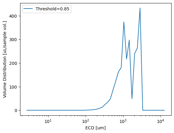
We can plot directly from xarray in exactly the same way as from the Pandas DataFrame (so it doesn’t matter which you use here). The benefit of ‘xstats’ as an xarray is that it now contains it’s own metadata

import matplotlib.pyplot as plt

dias, vd = pyopia.statistics.vd_from_stats(xstats, toml_steps['general']['pixel_size'])

plt.plot(dias, vd, label=f"Threshold={toml_steps['steps']['segmentation']['threshold']}")
plt.xscale('log')
plt.xlabel('ECD [um]')
plt.ylabel('Volume Distribution [uL/sample vol.]')
plt.legend()
plt.show()